AT3. New Quantum Mechanics
Bohr's idea that electrons are found in different orbitals or energy levels was an important step in understanding the structure of an atom. Louis de Broglie's particle-wave relationship was also a crucial development.
Werner Heisenberg and Erwin Schrodinger were able to take these ideas and develop modern quantum mechanics. The main significance of quantum mechanics is the ability to very accurately predict physical properties using basic mathematical principles. Heisenberg and Schrodinger used different kinds of mathematics to explain atomic structure, but they ultimately reached similar results.
The key approach by Schrodinger was to recognize the factors influencing the energy of an electron in an atom. He saw that there would be contributions from Coulomb's law, because of attractive forces between the electron and the nucleus as well as repulsive factors between different electrons. In addition, Schrodinger recognized that there would be a kinetic energy component related to the wavelength of the electron. Schrodinger combined these factors into "the Schrodinger wave equation."
Figure AT3.1. The factors Schrodinger accounted for in his wave equation.
Solving the wave equation is very useful. A solution to the equation, which is called a wave function, can indicate the energy of an electron in an atom. The solution can also be combined with other mathematical relations that will give specific predictions of different properties of atoms and molecules.
If you aren't familiar with how waves behave, you might start by looking here.
Problem AT3.1.
a) What happens to the energy of an electron as its wavelength gets shorter?
b) What happens to the energy of an electron as its wavelength gets longer?
c) If an electron is confined in a small space, what will happen to the electron's wavelength?
d) If an electron is allowed to expand into a large volume, what will happen to the electron's wavelength?
Apart from showing us the energy of the electron, the wavefunction carries other information. One additional item is the idea of phase. This idea is illustrated with a sine wave (although a wavefunction of an electron is a more complex, three-dimensional wave).
Figure AT3.2. A sine wave, showing phase and nodal properties.
One of the consequences of wave behaviour is the presence of nodes along a wave. A node is a place where the wave changes phase; in a sine wave, the wave goes from a "trough" or valley or negative phase to a "peak" or hill or positive phase. A node is also place where the amplitude of the wave is zero. For an electron, the amplitude of the wave is related to the chance of an electron being found at that position (you'll see more about that below). We wouldn't find an electron at a node, but it could be in one of the other positions along the wave.
Other important consequences of wave properties in electrons include interference behaviour. If two electrons are sent through parallel slits, a diffraction pattern results, like ripples from two different stones overlapping in a pond. That's because the waveforms of the two electrons interfere with each other. When the two waves overlap, they interact with each other in different ways, depending on whether they are in phase or out of phase.
Figure AT3.3. Constructive interference and wave addition.
If the waves are in phase with each other, constructive interference occurs, and a taller wave results. The peak of one wave adds onto the peak of another, and the trough of one wave falls into the trough of another. However, if the two waves are out of phase with each other, the peak of one falls into the trough of each other, and the wave disappears. That phenomenon is called destructive interference.
Figure AT3.4. Destructive interference and wave addition.
One of the funny consequences of quantum mechanics is that you don't need two different electrons to cause an interference pattern. A single electron can be sent through a pair of parallel slits and result in an interference pattern. The electron passes through both slits at the same time. Sometimes an electron does not behave like a solid particle at all.
The wave properties of electrons also become important when considering bonding between atoms. As atoms are brought together to share electrons, constructuve and destructive interference between electrons leads to different consequences in different situations. We will look at these factors in a later chapter.
We mentioned that mathematical operations are sometimes performed on the wavefunction in order to predict other properties. For example, if you want to get an idea of where an electron is, you have to square the wavefunction. You take the wavefunction and multiply it by itself.
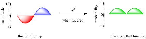
Figure AT3.5. The probability of finding an electron at a particular position is predicted by the square of the wavefunction.
We lose some information when we perform math on the wavefunction. We no longer have "amplitude"; instead we have a probability. The curve we see is a statistical distribution that tells us where the electron is most likely to be found (the highest point on the curve) as well as many other places where the electron might also be found (the rest of the curve). We no longer have phase information, either; when the negative portion of the wave was multiplied by itself, it gave a positive number.
Problem AT3.2.
What is the probability of finding an electron at a node?
It is useful to keep the idea of particle-wave duality in mind, for a number of reasons. When we think of an electron as a particle, like a tennis ball, it is easy to expect that it will behave like a real tennis ball. After all, we know where the tennis ball is; you can see it, right there. But if an electron is a wave, like a wave on the ocean, it is not really restricted to one location. First of all, it's spread out (maybe over many miles, in the case of some waves). Secondly, it doesn't sit still long enough for you to decide it's exactly here or there. That's a little more like an electron. Also, if you had two holes in a wall, you could only throw a tennis ball through one hole at once. If a wave splashed against the wall, though, it could pass through both holes at once.
So, instead of thinking of an electron as a ball, maybe we should think about it as a cup of water. There's a stiff wind blowing, so there are waves on the surface of the water. Also, there's no gravity, so we can take the cup away and the water will hold together there, with its waves. Of course, the electron is no more liquid than it is a solid, but we often need familiar analogies to remind us of these different aspects of something we can't really see.
When Schrodinger worked out solutions for his equation, he found evidence of quantization again. Bohr had found that the distance between the electron and nucleus was quantized. However, Schrodinger found four different electronic properties that were quantized. One of these properties of an electron, called the principle quantum number, corresponds roughly to Bohr's quantized distance from the nucleus.
Figure AT3.6. Schrodinger predicted that electrons should be found only at certain distances from the nucleus.
Two of the other properties have to do with the electron's direction from the nucleus. As it happens, a specific electron might be found in any direction from the nucleus. Alternatively, it might only be found in one direction or another.
Thinking in just two dimensions, suppose you have three tennis balls: a yellow one, a red one and a blue one. Imagine you are the nucleus of an atom and the tennis balls are electrons. In Bohr's model, the tennis balls might be found different distances away from you. Maybe one is five feet away, one is ten feet away, and one is twelve feet away. They cannot be found three feet away from you, or nine feet away or eleven feet away. They have to be found at those exact distances. However, they might be found in any direction: in front of you, behind you, to the left or right. They could all be lying in the same direction or all in different directions.
Figure AT3.7. Schrodinger predicted that particular electrons are found only in certain directions around the nucleus.
What Schrodinger's math seemed to be saying was that there was an additional restriction on where electrons could be found. In addition to a specific distance, the electron might be found only in certain directions from the nucleus. That direction relied on those other two quantized properties, called the magnetic and azimuthal quantum numbers. For one set of values, the electron could be found in any direction at all. For another set of values, though, the electron was restricted to lie along one particular axis.
In this model, maybe the yellow tennis ball has to be five feet way, but can be in any direction. But maybe the blue tennis ball has different quantum numbers. It is ten feet away and it can only be directly in front of you or directly behind you, but cannot be to your left or right. The red tennis ball, on the other hand, can only be found to your left or right, but never in front of you or behind you.
There is also a fourth quantum number, and it is called spin. Spin can't be described very well because it does not have an analogous big-world property such as distance or direction. However, it is an inherent property of an electron that can have either of two values. These values are sometimes called alpha and beta, or sometimes +1/2 and -1/2.
Despite the abstract nature of spin, it does have a real physical quality associated with it: if you place an electron in a magnetic field, it will interact differently with the magnetic field, depending on the value of its spin. Hence, spin is closely associated with magnetic properties of materials.
One of the basic rules of quantum mechanics is that no two electrons on the same atom can have the same two quantum numbers. You'll need some extra tennis balls to see how that works. Suppose you have two red balls, two yellow and two blue. The first yellow ball is found five feet away from you, in any direction. The second yellow tennis ball is also found five feet away from you and in any direction. So far, the yellow tennis balls have the same properties, so they must have different spin. Of course, you can't tell that they have different spins unless you put them in a very strong magnetic field, but you know they are different because you have faith that Schrodinger did his math correctly.
Figure AT3.8. Spin pairing allows two different electrons to be the same distance from the nucleus and along the same axis.
The two blue balls are ten feet away from you and they can only be found in front of you or behind you. It doesn't matter which. They could both be in front of you or both behind you or one in either direction. They also have two different spins.
Finally, the two red balls are also ten feet away from you, but they are found to your right or left (or both). They don't have to be a different distance away from you than the blue ones because they already have a different directional property, so we can repeat the distance property. The red balls also have two different spins, but you are having trouble telling which is which.
One more thing. The quantum world is a little more subtle than that. The quantum world also involves concepts such as the uncertainty principle. The uncertainty principle says it is difficult to find an electron's exact location. Instead, we work with probability. Instead of being five feet away exactly, we only know that the yellow ball has a very good chance of being five feet away. There is a slight chance it is four and a half feet away, and a very small chance it is only four feet away.
Similarly, the red tennis ball may not be exactly in front of you, although it is probably no more than a few feet to the left or right. The blue tennis balls may also be a few feet off their axis someplace. We can't predict exactly where they will be.
Problem AT3.3.
Let's do an exercise in pointillism. You will need a pencil, a ruler, and pens of four different colours. Gel pens work better than ballpoint pens. In a pinch, you could use crayons, coloured pencils or coloured markers.
a) Draw a line in pencil 6 cm long. Mark the midpoint of the line.
b) Draw a second line 6 cm long and perpendicular to the first line, so that the midpoints of the two lines intersect. You should have a nice X or cross with arms 3 cm long.
c) Lightly draw in dashed lines, 10 cm long, halfway in between the prvious lines, so that the midpoints of all the lines intersect. You should have a new X or cross with arms 5 cm long, superimposed on the old cross but rotated by 45 degrees.
d) Choose one of the solid lines to work on. Place two marks along that line, 1 cm away from the midpoint in each direction. Using the first pen, start putting dots on the paper, centered on one of those 1 cm points. Keep adding dots as you move away from that 1 cm point in all directions, but there should be fewer and fewer dots as you go out. Expand your dots the same distance in all directions. Try not to cross the dashed lines, however. Aim for about a hundred dots (or 50 if you aren't very patient or if you are using a marker). You should end with a roughly circular mass of dots, centered 1 cm from the midpoint; the mass should get fainter along its edges and heavier and darker towards its center.
e) Now do the same thing, using the same pen, at the other 1 cm point along the same line.
f) Now do the same thing, with a second pen, 1 cm away from the midpoint in both directions along the second solid line.
g) Now do the same thing, with a third pen, 3 cm away from the midpoint in both directions along the first solid line.
h) Now do the same thing, with a fourth pen, 3 cm away from the midpoint in both directions along the second solid line. You should end up with four pairs of coloured spots. Each spot should have higher value (heavier and darker) in the centre and should fade to lower value away from its centre.
What you have produced is a simplified, two-dimensional electron probability map. Each colour corresponds to a different "orbital", described by a set of principle, azimuthal and magnetic quantum numbers. Suppose your four colours describe the probability of finding a 2px, a 2py, a 3px and a 3py electron. With each dot, you sucessfully found the electron. The collection of dots tells you where a particular electron is most likely to be found; the highest value corresponds to the highest probability of locating an electron.
Compare and contrast your sets of dots with each other.
Problem AT3.4.
Construct another pointillist electron probability map, showing a two-dimensional slice through a 2s and 3s orbital in two different colours. Start with the same cross drawn in pencil, but this time when you put down dots with the first pen, centred 1 cm from the midpoint of the cross, don't restrict them along one line. Let them be any direction from the midpoint. Use a hundred dots. Add a second set of dots with the second pen, centred 3 cm from the midpoint of the cross, and in any direction from the midpoint. Compare and contrast the two sets of dots with each other, and with your previous map.
Why do electrons sort themselves out this way? One of the factors affecting electrons is electrostatic repulsion. They repel each other. To minimize that repulsion, the first pair of electrons might be a certain distance from the nucleus. A second pair may be a little farther away, so they're not too close to the first two. Once we reach a certain distance from the nucleus, electrons may be spread out enough that more than one pair could be found at that distance. Still, it is best to keep them a little farther away from each other. One pair may lie along one axis, and another pair may lie along a perpendicular axis. Of course, there is some repulsion between two electrons within the same pair, but the repulsion is actually decreased a little by having opposite spins (this is called spin pairing).
This site was written by Chris P. Schaller, Ph.D., College of Saint Benedict / Saint John's University (retired) with contributions from other authors as noted. It is freely available for educational use.
 Structure & Reactivity in Organic, Biological and Inorganic Chemistry
by Chris Schaller is licensed under a Creative Commons Attribution-NonCommercial 3.0 Unported License.
Structure & Reactivity in Organic, Biological and Inorganic Chemistry
by Chris Schaller is licensed under a Creative Commons Attribution-NonCommercial 3.0 Unported License.
Send corrections to cschaller@csbsju.edu
Navigation: